kNN/ANN #
The full name of the k-nearest neighbor algorithm is the k-nearest neighbors algorithm, abbreviated as kNN. It was first proposed in 1967, and the DOI of the paper is 10.1109/TIT.1967.1053964.
The kNN algorithm attempts to solve the following problem: given an n-dimensional vector dataset and a query vector Q, calculate the distance between Q and all the vectors in the dataset, and then find the k vectors (top k) that are closest to Q according to the distance.
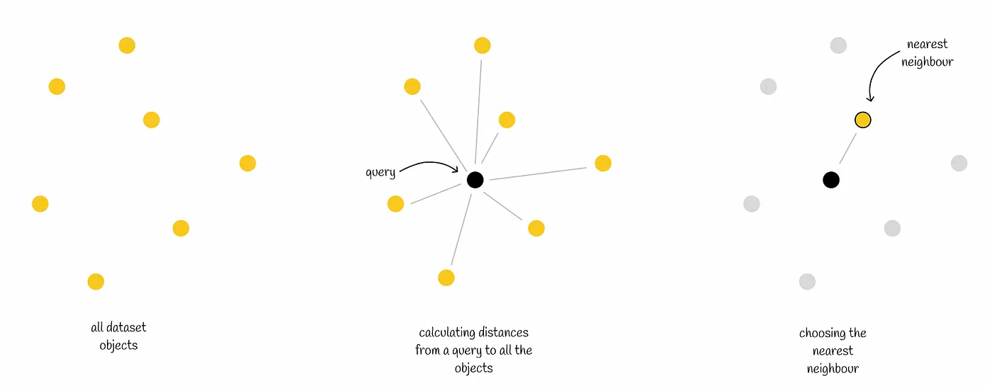
There are three points to note about the kNN algorithm
- Algorithm hyperparameters k
- Distance metric
- Sorting and querying topK
The kNN algorithm is a brute-force search that needs to iterate through all the data sets. The execution efficiency can be imagined in the case of large amounts of data. So there are two ways to sacrifice accuracy for time and space:
- Reduce the search range
- Reduce the vector dimension
This improved algorithm is called the Approximate Nearest Neighbor (ANN) algorithm. Two corresponding methods have been developed for the above two methods:
- By data set division, the search range is reduced, and the data structure in each subset can be a tree, graph, inverted index, etc.
- Use quantization (Quantization) to lossy compress high-dimensional vectors to reduce the amount of calculation when high-dimensional vectors are used. Product quantization (Product quantization) is often used.
Distance metric #
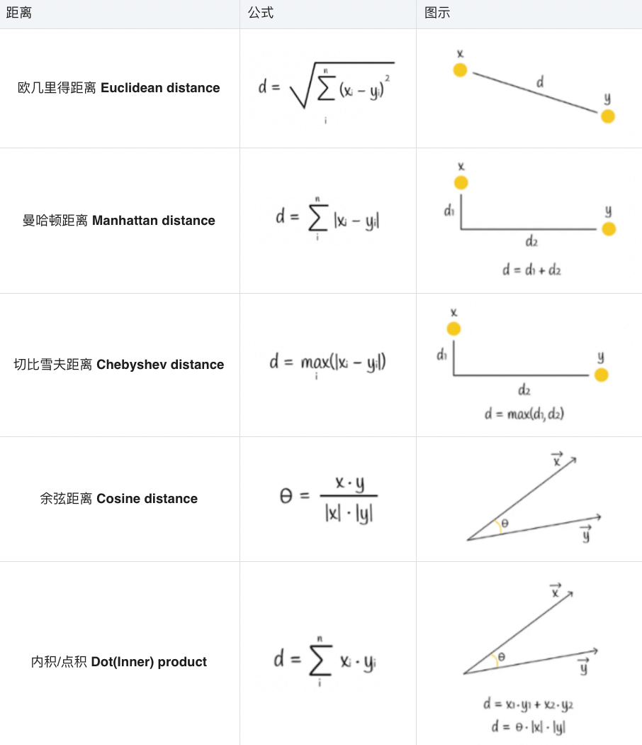
The distance metric determines the distance between vectors, which largely determines the division of space, the distance and ranking between candidate nodes and query nodes, etc. Here are the formulas for the five distance metrics
Vector quantization #
Vector quantization (Vector Quantization) compresses/encodes/transforms vectors into a shorter, more memory-efficient representation. Obviously, this is a form of lossy compression that improves ANN efficiency at the expense of accuracy. However, in practice, this loss of accuracy is permissible. Mathematically speaking, it is a means of vector discretization.
The most famous algorithm in vector quantization is product quantization (PQ, Product quantization)
Product quantization (Product quantization) #
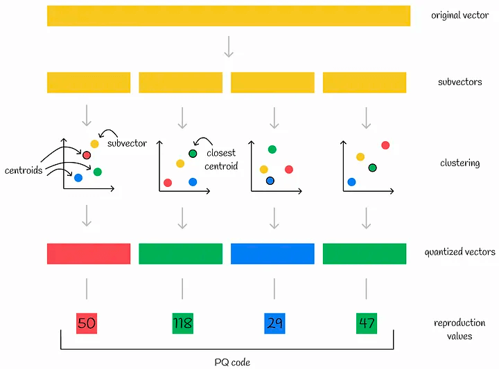
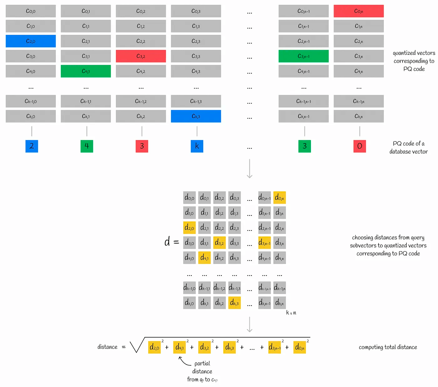
In the case of product quantization, for example, we first divide the vector into multiple subvectors. The subvectors of all vectors form a subspace, in which the K-means clustering algorithm is performed, and the centroid ID of the subspace closest to the subvector is recorded. The combination of the centroid IDs of all subvectors is the PQ code of a single vector.
After quantization, the vector is converted into n centroid IDs. Therefore, in order to store more efficiently, the number of centroid IDs, k, is often a power of 2, and the corresponding memory needs to store (n * log(k)\) bytes
Now that we have a quantized PQ code set, how do we perform an ANN search in the PQ code set?
Similarly, the query vector is divided into n sub-vectors, and the distance of each sub-vector to all the centroids in the corresponding subspace is stored in matrix form in d. We call each node in matrix d partial distances.
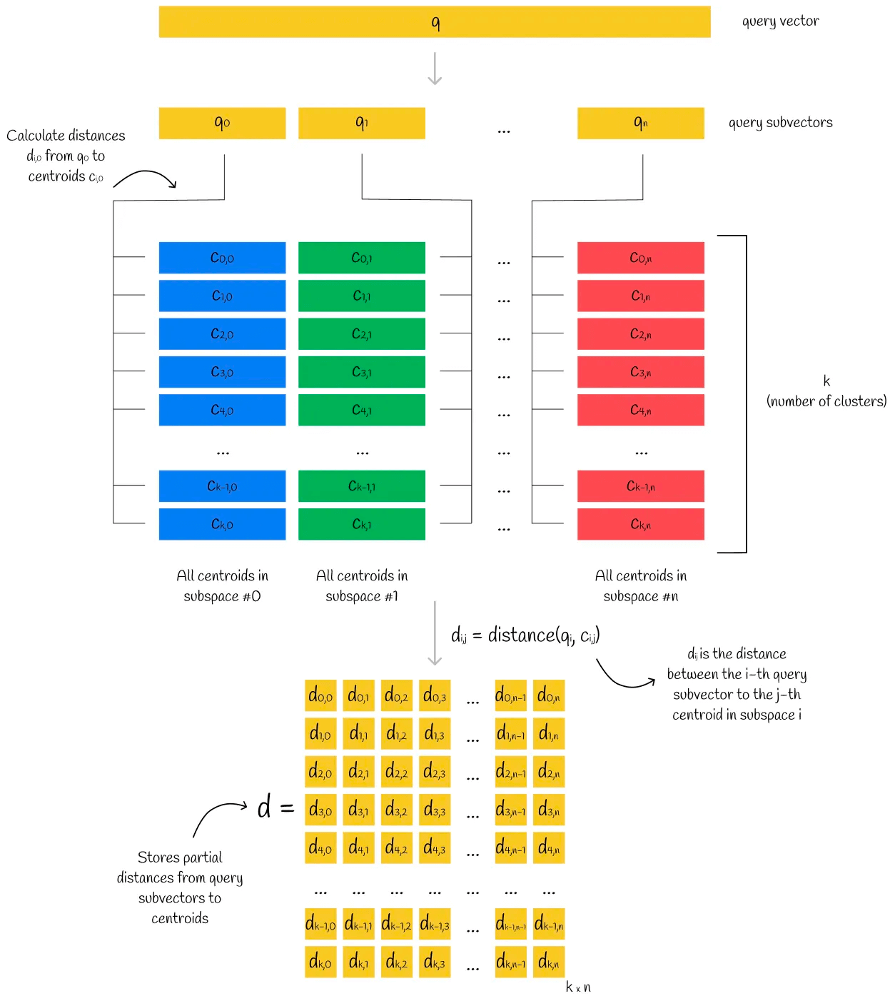
For the vectors in the dataset, we get the PQ code of each vector, and find the partial (relative) distance corresponding to the centroid in each subspace in the matrix d. In this way, we get n partial (relative) distances. Assuming that Euclidean calculation is used for this set of partial (relative) distances, the relative distance of the current sample to the query vector can be roughly calculated, and sorting according to this distance can get the topK.
The distance between the sample vector and the query vector calculated in this way is very close to the actual distance between the two vectors.
Data structure #
First, let’s talk about the implementation of the kNN algorithm. There are two main data structures for datasets: Linear and K-D Tree.
- Linear: maintains a linear array to hold all data
- K-D Tree: maintains all data in a k-dimensional binary tree
Implementing the ANN algorithm requires dividing into two dimensions: space division and data structure selection for nodes. There are many choices for data structures, including kd trees, inverted index IVF, graph HNSW, hash LSH, etc. We will explain each in turn.
Implementation based on KD-tree – take Annoy as an example #
Let’s first take a look at the data structure of the KD-tree. Here, we refer to golearn/kdtree/kdtree.go
type node struct {
    feature  int // -1: leaf, -2: nil
    value    []float64 // spatial vector, the spatial extent represented by this node
    srcRowNo int // the number of the axis perpendicular to the partition hyperplane
    left     *node // left subtree
    right    *node // right subtree
}

// Tree is a kdtree.
type Tree struct {
    firstDiv *node
    data     [][]float64 // data vector
}
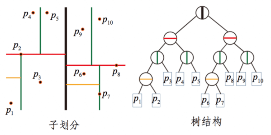
We mentioned that both kNN and ANN implementations can use kd trees. The biggest change in ANN is that a single tree is divided into multiple trees to improve execution efficiency. Annoy uses this idea to implement the ANN algorithm.
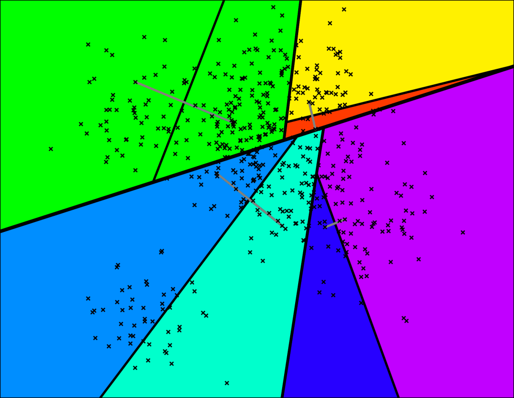
The idea behind Annoy is to randomly select two points in the entire n-dimensional space. These two points can be connected to form an n-1 dimensional hyperplane (hyperplane), and the normal plane of this hyperplane can divide the entire space into two parts. And so on. When I randomly select N pairs of points, there will be N normal planes, which can divide the entire space into 2N pieces, until the number of samples in the subspace is limited to K or less.
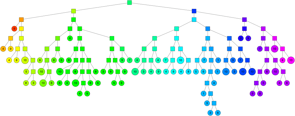
Each random split can construct a tree as shown in the figure below. We construct M groups of random splits in turn, so that we can get M trees, each of which contains all nodes. At this point, we have a forest.
The steps for searching are as follows
- Construct a priority queue based on the root nodes of all trees in the forest
- Find k neighborhood candidates in each tree
- Remove duplicate candidates
- Calculate the distance between all candidates after deduplication and the query vector
- Sort the candidates according to the distance
- Return topK
To summarize:
- In terms of space division, Annoy provides multiple partitions, each of which forms a tree. Each tree contains multiple subspaces cut according to the plane of the law, and each subspace maintains K nodes
- Each of the K nodes in each subspace is constructed using the K-D Tree method
- For distance selection, Annoy provides five types: Euclidean distance, Manhattan distance, cosine distance, Hamming distance and dot product distance
Finally, I highly recommend reading this article by Erik Bernhardsson, one of the developers of Annoy.
Nearest neighbors and vector models – part 2 – algorithms and data structures
Implementation based on IVF inverted index – taking Faiss as an example #
An inverted index is a common form of index. As the name suggests, it is a KV mapping of words/numbers to document IDs, as shown in the figure below. When performing a query, the hash function is used to calculate the value of the query, and then the corresponding mapping value is obtained from the hash table of the IVF index. The mapping value is usually a set of data, and then the topK nearest values in this set are queried. Faiss uses this data structure at the bottom.

Faiss (Facebook AI Search Similarity) is an ANN algorithm proposed by Facebook.
Two distance metrics are implemented in Faiss. The specific code is in faiss/IndexFlat.h:
- IndexFlatL2: Euclidean distance implementation
- IndexFlatIP: inner product implementation
For spatial partitioning, Faiss implements the K-means clustering algorithm:
- Randomly initialize k cluster centers (also called centroids)
- Calculate the distance of each sample to the centroids and assign the sample to the nearest centroid to form a cluster
- Then average the samples in each cluster to get a new set of cluster centroids; if the centroids have changed, repeat step 2 using the new set of centroids, otherwise go to the next step
- When the centroids no longer change, it means we have found relatively high-quality centroids
- Divide the space with these centroids and the samples belonging to the clusters, and we have obtained the Voronoi Diagram
When querying, we only need to find the nprobe centroids closest to the query vector, calculate and sort the distances between each sample in the candidate subspace and the query vector.
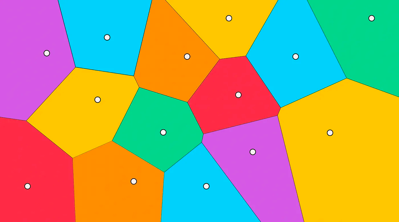
Let’s take a look at IVF inverted index. Faiss defines a header file to represent the basic implementation of IVF faiss/IndexIVF.h,
struct Level1Quantizer {
    Index* quantizer = nullptr; /// Quantizer for vector-inverted list mapping
    size_t nlist = 0; /// Number of inverted lists/Voronoi cells
}

struct IndexIVFInterface : Level1Quantizer {
    size_t nprobe = 1;    /// The number of probes during ANN queries, i.e. the number of regions required to determine the approximate candidate
  size_t max_codes = 0;
}

struct IndexIVF : Index, IndexIVFInterface {
    InvertedLists* invlists = nullptr; /// Pointer to inverted list
    int parallel_mode = 0; /// Whether to use OpenMP parallelism
}
The actual content of the inverted index is stored in InvertedLists, and the specific data structure is as follows
typedef int64_t faiss_idx_t; ///< all indices are this type
typedef faiss_idx_t idx_t;

struct InvertedLists {
    size_t nlist;     /// number of inverted indices
  size_t code_size; /// size of each vector code size per vector in bytes
  bool use_iterator;
}

/// implementation of an inverted list array (default)
struct ArrayInvertedLists : InvertedLists {
    std::vector<std::vector<uint8_t>> codes;
    std::vector<std::vector<idx_t>> ids;
}
IVFPQ #
We have seen how faiss partitions data. Combining this with the PQ quantization algorithm described earlier, we get IVFPQ. The specific steps are as follows
- For the entire vector space, find the centroid using K-means and divide it into n Voronoi cells
- For each sample in each Voronoi cell, calculate its relative distance to the centroid, i.e., use the centroid as point 0 to obtain the relative vector
- For each sample in each Voronoi cell, perform PQ product quantization on the relative vector, i.e., split the relative vector sample in the Voronoi cell into sub-vectors, cluster the sub-vector space to obtain the centroid, and convert the vector to PQ code
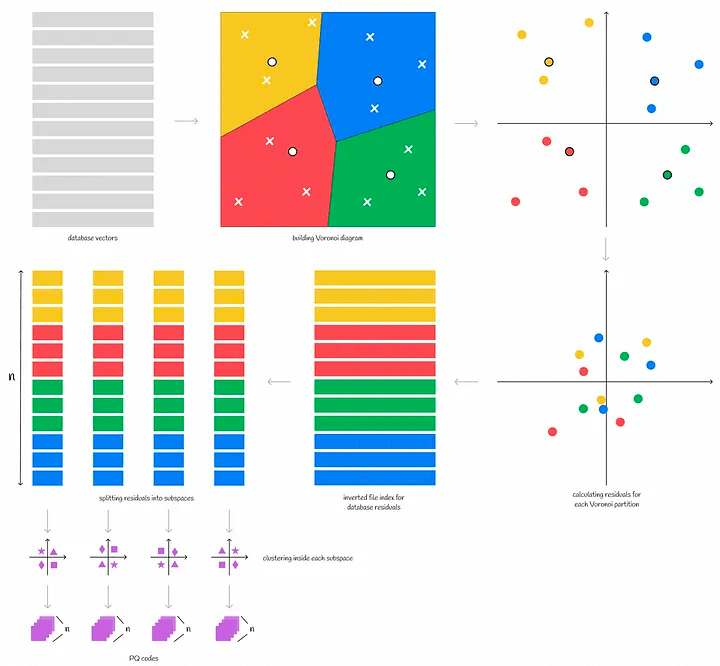
To summarize
- In terms of spatial partitioning, Faiss implements the K-means algorithm to select the centroid, and uses principal component analysis (PCA, principal components analysis) and product quantization (PQ, product quantization) to reduce the dimension and quantize the vectors
- For subspace storage, Faiss provides three methods: IVF inverted index, HNSW and LSH. Here, we mainly introduce IVF
- For distance measurement, Faiss implements two distances: Euclidean and inner product
Finally, Faiss’s documentation can be found at the following
Implementation based on HNSW graphs—using pgvector as an example #
HNSW is the full name of Hierarchical Navigable Small World (Hierarchical Navigable Small World).
Let’s first look at NWS, which is also known as a Delaunay graph: suppose there are X vector samples, each of which needs to be connected to M neighboring samples. During construction, the distance of each sample to all nodes in the current graph is calculated in turn, and M nodes are connected.
When searching, a greedy algorithm is used. A node is selected as the head node, and the distances from the head node and its connected nodes to the query node are calculated. If the head node is the closest, the current head node is its nearest neighbor, otherwise a closer node is selected and the above steps are repeated.
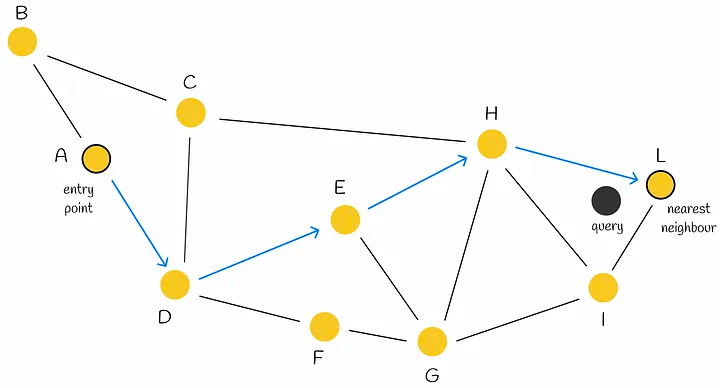
HNSW is a hierarchical version of NSW, which borrows the idea of skip-lists. The only difference is that skip-lists are used to hierarchize linked lists, while HNSW is used to hierarchize NSW graphs.
When constructing HNSW, the most important issue is how to determine the layer number of a node, which is also the most important issue when constructing NSW.
The HNSW paper proposes a formula for calculating the level of each inserted node. Where (m_L) is the normalization factor, the larger the value, the larger the value of (l), which represents the greater the probability of the node appearing in a higher layer; and L is the maximum number of layers.
$$ l = L - ln(unif(0..1)) *m _L $$
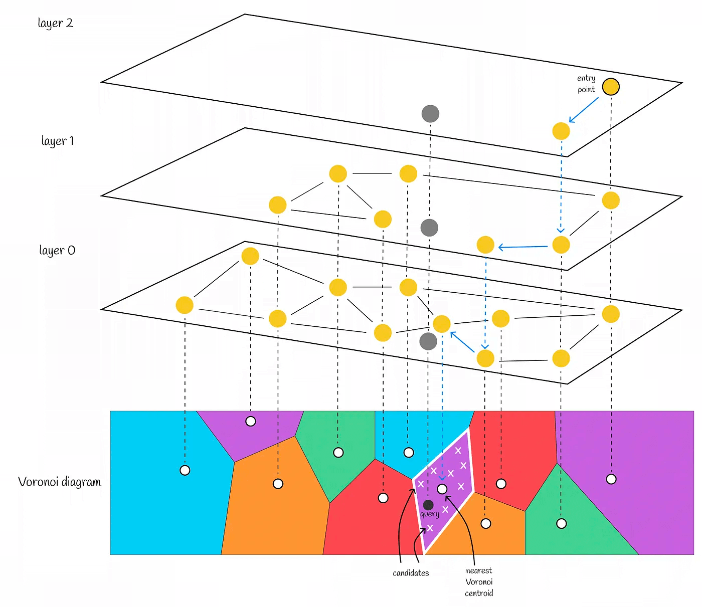
During the query, starting from the head node at the top layer, find the neighbor node that is closest to the query node, until the node closest to the query node at the current layer is found, then go to the next layer to query, and so on, until the 0th layer is queried, and the nearest neighbor node can be found.
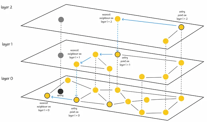
pgvector The ANN algorithm implemented with this data structure, pgvector provides the ANN approximate query capability as a PostgresSQL plug-in. First, let’s take a look at the data structure defined in the code
// Vector
typedef struct Vector
{
   int32     vl_len_;      /* varlena header (do not touch directly!) */
   int16     dim;         /* number of dimensions */
   int16     unused;
   float     x[FLEXIBLE_ARRAY_MEMBER];
}         Vector;

// Node
typedef struct HnswElementData
{
   List      *heaptids;
   uint8     level;  // layer number
   HnswNeighborArray *neighbors; // array of neighbors
   BlockNumber blkno; // block number
   OffsetNumber offno;  // offset number
   Vector    *vec;  // vector
}         HnswElementData;

typedef struct HnswMetaPageData
{
   uint32    magicNumber;
   uint32    version; // version
   uint32    dimensions; // dimensions
   uint16    m; //
   uint16    efConstruction;
   BlockNumber entryBlkno; // entry block number
   OffsetNumber entryOffno; // entry offset
   int16     entryLevel; // entry level
   BlockNumber insertPage;
}         HnswMetaPageData;

typedef HnswMetaPageData * HnswMetaPage;
Next, let’s look at how to assign layers to nodes in pgvector
#define HNSW_DEFAULT_M  16

// optimal ML value
#define HnswGetMl(m) (1 / log(m))
// calculate maximum level
#define HnswGetMaxLevel(m) Min(((BLCKSZ - MAXALIGN(SizeOfPageHeaderData) - MAXALIGN(sizeof(HnswPageOpaqueData)) - offsetof(HnswNeighborTupleData, indextids) - sizeof(ItemIdData)) / (sizeof(ItemPointerData)) / m) - 2, 255)

// Random number between 0 and 1
#if PG_VERSION_NUM >= 150000
#define RandomDouble() pg_prng_double(&pg_global_prng_state)
#else
#define RandomDouble() (((double) random()) / MAX_RANDOM_VALUE)
#endif

/*
 * Maximum number of connections to the upper level of each node
 */
int HnswGetM(Relation index)
{
    HnswOptions *opts = (HnswOptions *) index->rd_options;

    if (opts)
       return opts->m;

    return HNSW_DEFAULT_M;
}

// Initialize node
HnswInitElement(ItemPointer heaptid, int m, double ml, int maxLevel)
{
    HnswElement element = palloc(sizeof(HnswElementData));

    // Calculate the number of layers
    int          level = (int) (-log(RandomDouble()) * ml);

    if (level > maxLevel)
       level = maxLevel;

    element->level = level;
    ...
}
pgvector also implemented an IVF-based ANN implementation at the beginning, but this part will not be discussed in detail.
IVF-HNSW #
In the 2018 paper [Revisiting the Inverted Indices for Billion-Scale Approximate Nearest Neighbors] (https://github.com/dbaranchuk/ivf-hnsw), a HNSW + IVF method is proposed, which is said to be able to handle ANN queries for billion-scale vector data. The main points are as follows:
- Use HNSW to spatially partition the dataset, and divide the dataset into multiple regions through a hierarchical structure. The nodes in HNSW correspond to a centroid, and a centroid represents a subspace.
- For each subspace, there is an IVF index to store all the vectors belonging to it
- PQ encode the vectors in the IVF index to quantize the vectors
LSH-based implementation – FALCONN as an example #
LSH stands for Local Sensitive Hashing.
As the name suggests, it narrows down the search scope by converting data vectors into hash values, with neighboring nodes meaning more likely to collide. The LSH algorithm mainly consists of three steps:
-
Shingling: Use k-gram to split the text into sequences of k consecutive characters, and then encode each sequence using the one-hot algorithm to complete the conversion of the text into a vector.

-
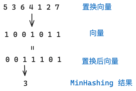
MinHashing: Convert the vector obtained by shingling into a “signature” (signature). The main purpose of this step is to convert the vector to a smaller dimension (MinHashing). This signature can preserve the similarity of its samples.
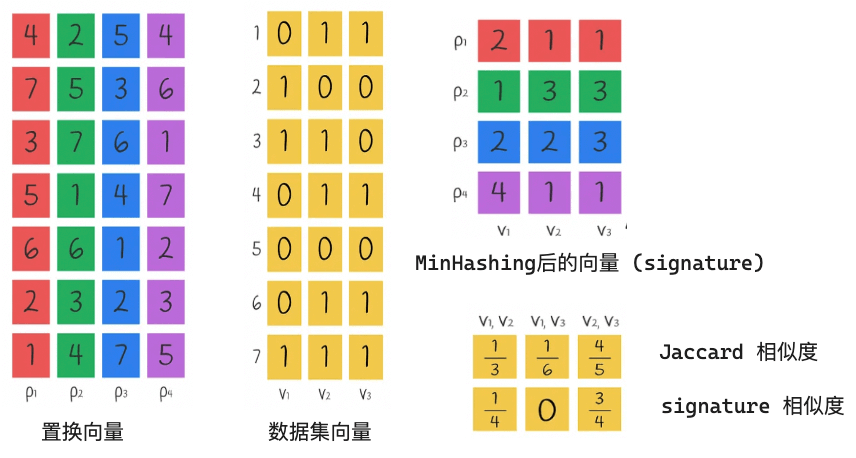
For this step, we first need to randomly generate multiple permuting vectors. The MinHashing method will permute the permuting vector and the sample vector, and return the index of the first one that is equal to 1 after permutation. As shown in the figure below, we use one permuting vector, and the vector will get 3 after passing through MinHashing.
Next, we use multiple permutation vectors and then obtain the value after MinHashing for each vector. We then perform signature similarity and Jaccard similarity on this value, as shown in the figure below:
Finally, we will explain the calculation of signature similarity and Jaccard similarity. Take the pair of vectors V1 and V2 as an example
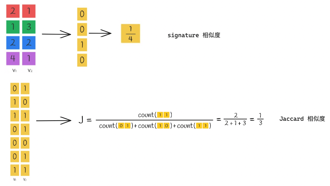
We can see that the similarity calculated by the signature is roughly equal to the Jaccard similarity, which means that we can convert the vectors into signatures and then calculate their similarity, which is more efficient than calculating the similarity directly using the Jaccard Index through the original vectors!
-
LSH function: The LSH method hashes the signature block into different buckets.
First, the signature is split into equal parts, each of which is called a band, and each band contains r values. For example, if the signature has 9 values, it is split into 3 groups of 3, so there are 3 bands, each with 3 values.
Then each band is hashed and mapped to a separate bucket. If the signature is split into n parts, there will be n buckets.
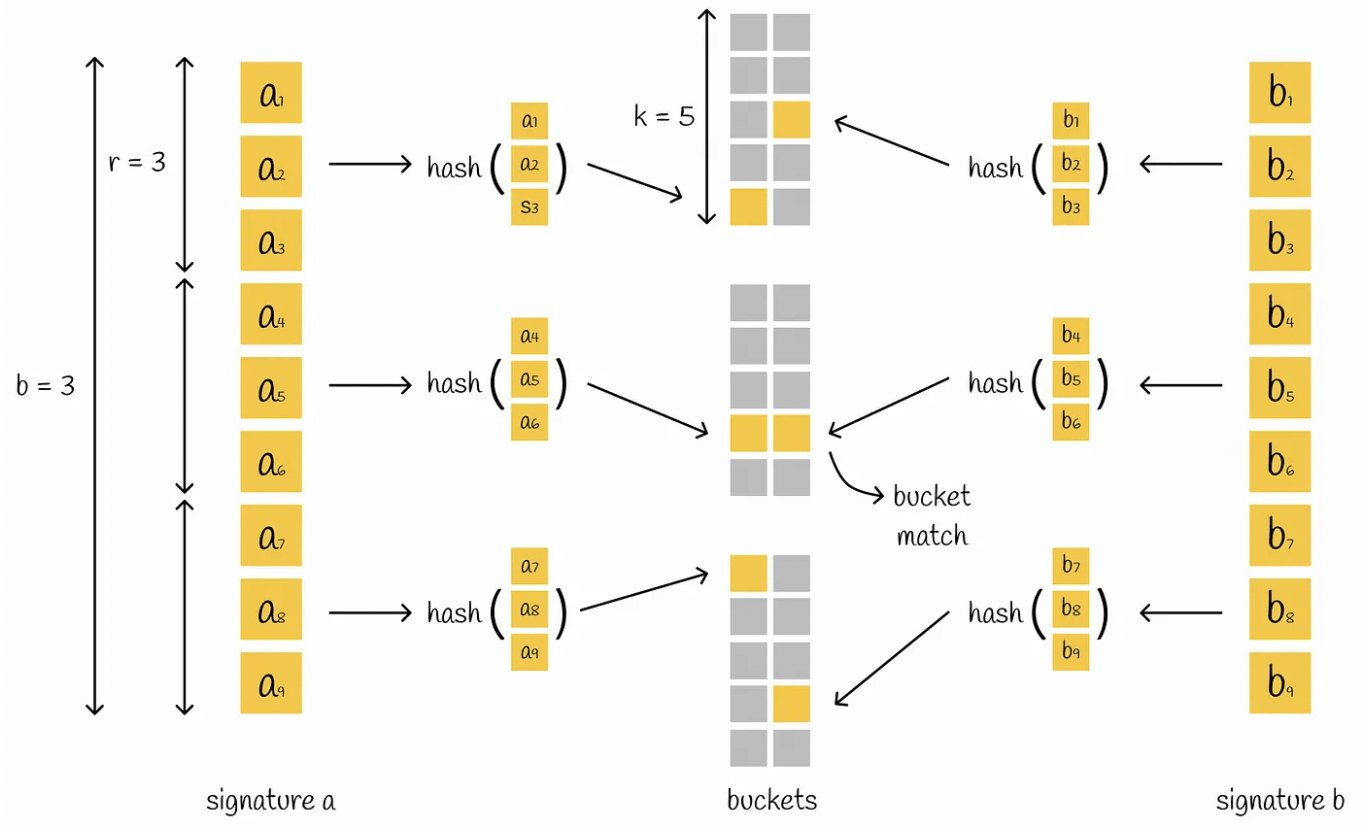
Recall that we use Shingling to convert text → vector, then call MinHashing to convert vector → signature, and finally use the LSH method to hash the signature segments and store them in different buckets.
When querying, we only need to convert the query into a vector, calculate the signature, hash the signature, find the value in the bucket corresponding to the hash, get the corresponding vector, and the vector that has the most hash collisions with the vector represents the nearest neighbor node.
Now let’s think about the meaning of LSH local sensitive hashing in reverse. Local means that the signature is split, and sensitive refers to the hash collision in each split bucket. This leads to what we said at the beginning and at the end: the more times the signature hash collides, the higher the similarity with the query vector.
FALCONN has officially implemented this idea of the LSH algorithm, but I won’t describe it in detail here (I’m lazy). The specific project address is FALCONN, and the wiki in the project is more recommended to read LSH-Primer.
Extension 1: ANN benchmarking #
Finally, I recommend a website that collates benchmarking results for most mainstream ANN algorithms
Extension 2: Data vectorization #
The previous section mainly introduced how to query topk when we have a vectorized dataset. Here is a brief introduction to how to vectorize data.
Take text vectorization as an example. Vectorization methods include the bag-of-words model, TF-IDF, co-occurrence matrix, word embedding, etc. The most commonly used method is word embedding. The algorithm principle can be found in NLP–Text Vectorization.
The following models are currently implemented based on word embedding:
| Model | Project/document address |
|---|---|
| M3E (Moka Massive Mixed Embedding) | https://github.com/wangyuxinwhy/uniem |
| BGE (baai general embedding) | https://github.com/FlagOpen/FlagEmbedding |
| text-embedding-ada-002 | https://cloud.baidu.com/doc/WENXINWORKSHOP/s/alj562vvu |
| 文心 Embedding | https://cloud.baidu.com/doc/WENXINWORKSHOP/s/alj562vvu |
| glm text embedding | https://open.bigmodel.cn/dev/api#text_embedding |
| RoPE (rotary-embedding) | https://github.com/ZhuiyiTechnology/roformer |
| LlamaCppEmbeddings | https://github.com/ggerganov/llama.cpp/blob/master/examples/embedding/embedding.cpp |
| text2vec | https://github.com/shibing624/text2vec |
Seeing this, we can naturally associate that text data can be quantized, and images, documents, statistical data, etc. can of course also be quantized, so ANNs are also applicable in these scenarios.
References #
List: Similarity Search | Curated by Vyacheslav Efimov | Medium
Nearest neighbors and vector models – part 2 – algorithms and data structures

